同构或非同构 (isomorphic)

import networkx as nx
import numpy as np
import matplotlib.pyplot as plt

图同构是一个非常有趣的话题，在图论和网络科学中有着广泛的应用 — 请查看同构教程以获得更深入的介绍！

确定两个图 G 和 H 是否同构，本质上归结为在 G 和 H 的节点之间分别找到有效的同构映射。找到这种映射的过程可能相当耗时。让我们用一对基本图来探究。

G = nx.complete_graph(100)
H = nx.relabel_nodes(G, {n: 10 * n for n in G})

我们先验地知道 G 和 H 是同构的，因为 H 只是 G 的一个节点重新标记的副本。当然，我们可以验证这一点

nx.is_isomorphic(G, H)

True

并进行一些基本计时，了解确定所需的时间

%timeit -n1 -r1 nx.is_isomorphic(G, H)

72.1 ms ± 0 ns per loop (mean ± std. dev. of 1 run, 1 loop each)

还不错，至少对于这些相对较小且简单的图来说 - 但绝对计时值并没有特别大的参考意义。与一个非常相似但图 非同构 的例子相比，情况如何？

H_ni = G.copy()
H_ni.remove_edge(27, 72)  # Remove a single arbitrary edge

同样，我们先验地知道 G 和 H_ni 非同构

nx.is_isomorphic(G, H_ni)

False

但即使我们所做的只是从 H 中移除一条任意的边，同构判断的速度却快了几个数量级！

%timeit -n1 -r1 nx.is_isomorphic(G, H_ni)

92.8 μs ± 0 ns per loop (mean ± std. dev. of 1 run, 1 loop each)

定量分析

import timeit

iso_timing, non_iso_timing = (
    timeit.timeit(f"nx.is_isomorphic(G, {G2})", number=20, globals=globals())
    for G2 in ("H", "H_ni")
)
print(f"Relative compute time, iso/non_iso example: {iso_timing/non_iso_timing:.2f}")

Relative compute time, iso/non_iso example: 1104.39

表面上看，两个如此相似的情况会导致计算时间如此巨大的差异，这似乎令人惊讶。

证明两个图同构的唯一方法是在它们之间找到有效的同构映射 — 在最坏的情况下，这可能需要搜索 G 和 H 之间节点 所有可能的 映射！然而，是 同构的图则保证具有某些属性。例如，同构图必须具有相同的度分布。如果两个图被证明具有 不同 的度分布，那么我们可以明确地说它们 非同构，而无需测试 G 和 H 之间的任何一个潜在节点映射。然而 - 仅仅证明两个图具有相同的度分布并不足以证明它们是同构的！

这种不对称性是 nx.could_be_isomorphic 函数的动机，该函数比较图对的各种属性，以确定它们是否，嗯，可能 同构。图有很多属性可以比较，从简单的（即节点数量）到更复杂的特征，如平均聚类系数。nx.could_be_isomorphic 有四种内置属性检查

1. 图的阶数（即节点数量）

2. 每个节点的度

3. 图中每个节点所属的三角形数量

4. 图中每个节点所属的最大团数量

探索图谱上的属性

所以 - 我们有一些图的属性，可以用来判断两个图是否 可能 同构。我们也知道有些属性计算起来比其他属性更耗时。那么一个显而易见的问题是：这些各种属性在过滤非同构图方面有多“好”？例如，如果在绝大多数情况下仅凭度分布就足以证明两个图非同构，那么一个好的经验法则是先在 could_be_isomorphic 中测试度分布，因为度分布计算起来非常快（相比于三角形或团）。

普遍回答这个问题可能不太可能，但也许我们可以通过在一组可管理的图上探索这个问题来建立一些直觉。例如，我们可以使用 nx.graph_atlas_g 在所有具有 7 个节点的完全连通简单图上调查这些属性。

atlas = nx.graph_atlas_g()[209:]  # Graphs with 7 nodes start at idx 209
print(f"{len(atlas)} graphs with 7 nodes.")

# Limit analysis to fully-connected graphs
atlas = [G for G in atlas if nx.number_connected_components(G) == 1]
print(f"{len(atlas)} fully-connected graphs with 7 nodes.")

1044 graphs with 7 nodes.
853 fully-connected graphs with 7 nodes.

现在让我们检查这些图的属性。让我们定义一些属性提取的快捷方式来节省一些打字工作

from itertools import chain
from collections import Counter

degree = lambda G: sorted(d for _, d in G.degree())
triangles = lambda G: sorted(nx.triangles(G).values())
cliques = lambda G: sorted(Counter(chain.from_iterable(nx.find_cliques(G))).values())

# Map each callable to a more detailed name - this will be useful for e.g.
# labeling plots
name_property_mapping = {
    "degree distribution": degree,
    "triangle distribution": triangles,
    "maximal clique distribution": cliques,
}

从这里，让我们互相比较这些图！最简单的方法就是暴力地将每个图与其他图进行比较

def property_matrix(property):
    """`property` is a callable that returns the property to be compared."""
    return np.array(
        [[property(G) == property(H) for H in atlas] for G in atlas],
        dtype=bool,
    )

让我们先做一些健全性检查。根据图谱的定义，我们期望 没有 任何一个图与其他图同构（除了与自身）。如果我们将这个期望转化为我们的 property_matrix，我们期望 isomorphic 属性矩阵是一个单位矩阵 - 即只有对角线上的值是 True。

is_iso = np.array([[nx.is_isomorphic(G, H) for H in atlas] for G in atlas], dtype=bool)
np.array_equal(is_iso, np.eye(len(atlas), dtype=bool))

True

健全性检查通过 — 现在让我们继续属性比较

import time

p_mats = []
for name, property in name_property_mapping.items():
    # Do some (very) rough timing of the property computation
    tic = time.time()
    pm = property_matrix(property)
    toc = time.time()
    print(f"{toc - tic:.3f} sec to compare {name} for all graphs")
    p_mats.append(pm)

# Unpack results
same_d, same_t, same_c = p_mats

3.995 sec to compare degree distribution for all graphs

38.882 sec to compare triangle distribution for all graphs

52.182 sec to compare maximal clique distribution for all graphs

让我们先看看大致的计时。再次强调，我们必须谨慎得出普遍结论，因为我们只处理了如此小的图子集。[1] 尽管如此，我们注意到计算/比较度分布比 cliques 或 triangles 大约快一个数量级，而这两者（至少对于这些图来说）计算时间处于同一数量级。

属性本身如何？

fig, ax = plt.subplots(1, 3, figsize=(9, 3))

for a, pname, pm in zip(ax, name_property_mapping, p_mats):
    a.imshow(pm, cmap=plt.cm.Blues)
    a.set_title(pname)

ax[1].set_xlabel("atlas idx (H)")
ax[0].set_ylabel("atlas idx (G)")
fig.tight_layout()

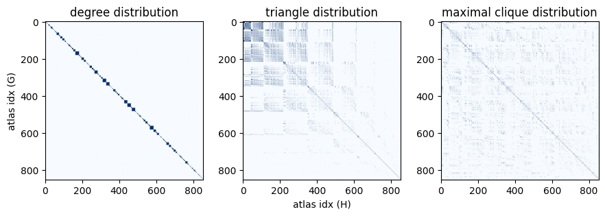
一件立即引起注意的事情是，所有具有相同度分布的图似乎被组织在一起，彼此相邻。仔细查看 nx.graph_atlas_g 的文档字符串（docstring）可以解释原因：度序列是图谱中图的排序依据之一。

我们可能注意到的另一件事是，具有相同三角形分布的图对集中在矩阵的左上角。这也有道理 — 图谱是根据（除其他外）递增的度序列排序的。因此，索引最低的图在度序列中具有最小值。一个三角形需要 至少 3 个节点 具有至少 2 的度 — 这意味着矩阵的左上角包含了所有没有三角形的图对，而三角形出现的倾向性通常随着度分布的增加而增加（从左上到右下）。

让我们对结果进行量化。在这 853 个具有 7 个节点的完全连通图中，有多少个具有相同的属性？我们可以对属性掩码求和来回答这个问题，但必须记住

1. 忽略对角线，即不包括每个图与自身的比较，以及

2. 我们在属性计算中偷懒了，最终将每个图互相比较了两次（即 G 与 H，以及 H 与 G），所以我们也需要考虑到这一点。

import pandas as pd

num_same = {
    f"Same {pname}": (pm & ~is_iso).sum() // 2
    for pname, pm in zip(name_property_mapping, p_mats)
}

# Use pandas to get a nice html rendering of our tabular data
pd.DataFrame.from_dict(num_same, orient="index")

	0
相同的度分布	3048
相同的三角形分布	9696
相同的最大团分布	6437

我们也可以查看属性的组合 - 例如：具有相同度分布 和 三角形分布的图的数量

same_dt = same_d & same_t & ~is_iso
print(
    f"Number of graph pairs with same degree and triangle distributions: {same_dt.sum() // 2}"
)

Number of graph pairs with same degree and triangle distributions: 270

这是一个相当强的过滤器！具有 7 个节点的完全连通图的非同构对总数为：\(\frac{853^{2} - 853}{2} = 363378\)。仅通过度、三角形或团进行过滤会产生数千个候选对象，但结合属性可以形成更强的过滤器，用于确定图是否 可能 同构。

让我们看看其中的一些图对。

candidates = zip(*np.where(same_dt))

# Filter out the duplicates
graph_pairs = []
seen = set()
for pair in candidates:
    if pair[::-1] not in seen:
        graph_pairs.append(pair)
        seen.add(pair)

fig, ax = plt.subplots(1, 2, figsize=(9, 3))

# First pair of graphs with same degree and triangle distributions
pair = graph_pairs[0]
G, H = (atlas[idx] for idx in pair)

for idx, a in zip(pair, ax):
    G = atlas[idx]
    nx.draw(G, ax=a)
    a.set_title(f"atlas[{idx}]\ndegree: {degree(G)}\ntriangles: {triangles(G)}")
fig.tight_layout()

nx.could_be_isomorphic(G, H, properties="dt")

True

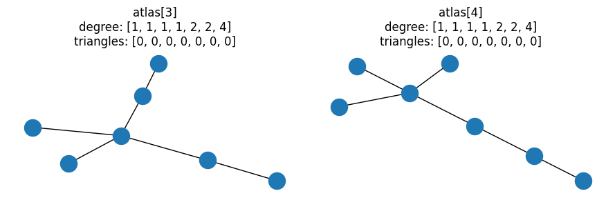
这符合我们的预期，很好地说明了仅检查属性不足以证明图同构。不过，由于没有三角形，这有点无聊 - 让我们看看包含三角形的图对

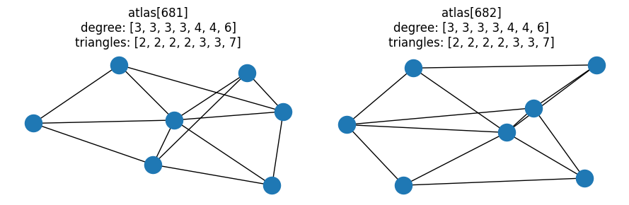
fig, ax = plt.subplots(1, 2, figsize=(9, 3))

# Last pair of graphs with same degree and triangle distributions
pair = graph_pairs[-1]

for idx, a in zip(pair, ax):
    G = atlas[idx]
    nx.draw(G, ax=a)
    a.set_title(f"atlas[{idx}]\ndegree: {degree(G)}\ntriangles: {triangles(G)}")
fig.tight_layout()

让我们进一步细化我们的调查 — 在 363378 对可能的图对中，有多少对具有相同的组合度-三角形分布，但具有 不同 的团分布？换句话说，对于多少图对来说，最大团的分布是决定这些图是否可能同构的决定性因素？

让我们首先结合独立计算的属性掩码来约束搜索空间

diff_c = same_d & same_t & ~same_c & ~is_iso

print(
    "Number of graph pairs with same degree and triangle distributions\n"
    f"but different clique distributions: {diff_c.sum() // 2}"
)

candidates = zip(*np.where(diff_c))

# Filter out the duplicates
graph_pairs = []
seen = set()
for pair in candidates:
    if pair[::-1] not in seen:
        graph_pairs.append(pair)
        seen.add(pair)

Number of graph pairs with same degree and triangle distributions
but different clique distributions: 107

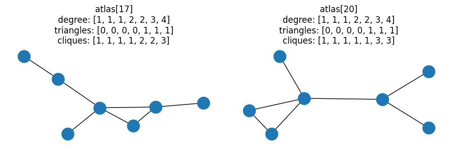
这是这些候选对中“最简单”的一对，即具有最低度序列的图对

fig, ax = plt.subplots(1, 2, figsize=(9, 3))

# Last pair of graphs with same degree and triangle distributions
pair = graph_pairs[0]

for idx, a in zip(pair, ax):
    G = atlas[idx]
    nx.draw(G, ax=a)
    a.set_title(
        f"atlas[{idx}]\ndegree: {degree(G)}\ntriangles: {triangles(G)}\ncliques: {cliques(G)}"
    )
fig.tight_layout()

至此，我们将所有可能的 7 节点完全连通图组合过滤到剩下 107 个具有相同度分布、三角形分布但 不同 团分布的候选对。然而 - 回想一下，到目前为止，我们仅 独立地 比较了这些属性 - 即，我们比较了排序后的度序列，然后是排序后的三角形分布等等。这比我们考虑节点的 组合 属性要宽松。换句话说，与其只比较度然后比较三角形 - 如果我们计算 每个节点 的度 和 三角形数量，然后根据这种组合的度-三角形数量特征对节点进行排序呢？could_be_isomorphic 比较组合属性，所以我们可以通过将其应用于我们的候选对来回答我们的问题。

# All graph pairs that have the same *combined* degree-and-triangle distributions
# but a different clique distributions
resulting_pairs = [
    (int(G), int(H))
    for (G, H) in graph_pairs
    if nx.could_be_isomorphic(atlas[G], atlas[H], properties="dt")
]
resulting_pairs

[(318, 325), (473, 479)]

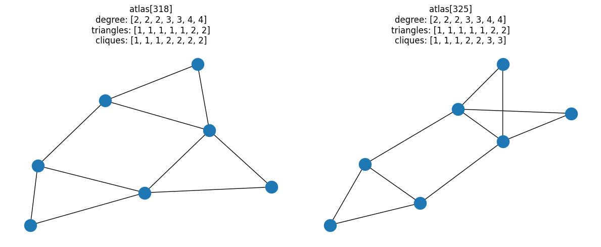
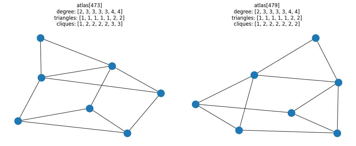
在所有具有 7 个节点的完全连通图中，只有两对唯一的图具有相同的度-三角形组合属性，但具有不同的团分布。

for i, pair in enumerate(resulting_pairs):
    fig, ax = plt.subplots(1, 2, figsize=(12, 5))

    for idx, a in zip(pair, ax):
        G = atlas[idx]
        nx.draw(G, ax=a)
        a.set_title(
            f"atlas[{idx}]\ndegree: {degree(G)}\ntriangles: {triangles(G)}\ncliques: {cliques(G)}"
        )
    fig.tight_layout()

启发

您可能想知道是什么激发了这条特定的调查路线。这项分析最初是为了找到 nx.could_be_isomorphic 的测试用例而进行的。

[1]

随着图变大，它们捕获的关系的复杂性也会大大增加！