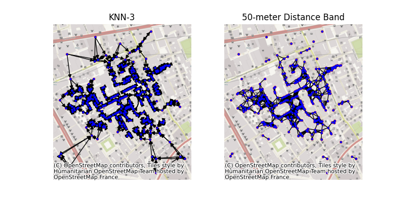
从地理点构建图

此示例展示了如何使用 PySAL 和 geopandas 从一组点构建图。在此示例中，我们将使用约翰·斯诺 (John Snow) 于 1853 年记录的著名的布罗德街水泵霍乱病例集。此处展示的方法也可以直接处理多边形数据，将其质心用作代表点。

from libpysal import weights, examples
from contextily import add_basemap
import matplotlib.pyplot as plt
import networkx as nx
import numpy as np
import geopandas

# read in example data from a geopackage file. Geopackages
# are a format for storing geographic data that is backed
# by sqlite. geopandas reads data relying on the fiona package,
# providing a high-level pandas-style interface to geographic data.
cases = geopandas.read_file("cholera_cases.gpkg")

# construct the array of coordinates for the centroid
coordinates = np.column_stack((cases.geometry.x, cases.geometry.y))

# construct two different kinds of graphs:

## 3-nearest neighbor graph, meaning that points are connected
## to the three closest other points. This means every point
## will have exactly three neighbors.
knn3 = weights.KNN.from_dataframe(cases, k=3)

## The 50-meter distance band graph will connect all pairs of points
## that are within 50 meters from one another. This means that points
## may have different numbers of neighbors.
dist = weights.DistanceBand.from_array(coordinates, threshold=50)

# Then, we can convert the graph to networkx object using the
# .to_networkx() method.
knn_graph = knn3.to_networkx()
dist_graph = dist.to_networkx()

# To plot with networkx, we need to merge the nodes back to
# their positions in order to plot in networkx
positions = dict(zip(knn_graph.nodes, coordinates))

# plot with a nice basemap
f, ax = plt.subplots(1, 2, figsize=(8, 4))
for i, facet in enumerate(ax):
    cases.plot(marker=".", color="orangered", ax=facet)
    try:  # For issues with downloading/parsing basemaps in CI
        add_basemap(facet)
    except:
        pass
    facet.set_title(("KNN-3", "50-meter Distance Band")[i])
    facet.axis("off")
nx.draw(knn_graph, positions, ax=ax[0], node_size=5, node_color="b")
nx.draw(dist_graph, positions, ax=ax[1], node_size=5, node_color="b")
plt.show()